Home
/
Blog
/
Developer Insights
/
Data visualization for beginners - Part 2

Data visualization for beginners - Part 2

Author
Shubham Gupta
Calendar Icon
May 16, 2018
Timer Icon
3 min read
Share

Welcome to Part II of the series on data visualization. In the last blog post, we explored different ways to visualize continuous variables and infer information. If you haven’t visited that article, you can find it here.In this blog, we will expand our exploration to categorical variables and investigate ways in which we can visualize and gain insights from them, in isolation and in combination with variables (both categorical and continuous).

Before we dive into the different graphs and plots, let’s define a categorical variable. In statistics, a categorical variable is one which has two or more categories, but there is no intrinsic ordering to them, for example, gender, color, cities, age group, etc. If there is some kind of ordering between the categories, the variables are classified as ordinal variables, for example, if you categorize car prices by cheap, moderate and expensive. Although these are categories, there is a clear ordering between the categories.

# Importing the necessary libraries.  
import numpy as np  
import pandas as pd  
import seaborn as sns  
import matplotlib.pyplot as plt  
%matplotlib inline  

We will be using the Adult data set, which is an extraction of the 1994 census dataset. The prediction task is to determine whether a person makes more than 50K a year. Hereis the link to the dataset. In this blog, we will be using the dataset only for data analysis.

# Since the dataset doesn't contain the column header, we need to specify it manually.   
cols = ['age', 'workclass', 'fnlwgt', 'education', 'education-num', 'marital-status', 'occupation', 'relationship', 'race', 'gender', 'capital-gain', 'capital-loss', 'hours-per-week', 'native-country', 'annual-income']  

# Importing dataset   
data = pd.read_csv('adult dataset/adult.data', names=cols)  
# The first five columns of the dataset.   
data.head()  

Bar graph

A bar chart or graph is a graph with rectangular bars or bins that are used to plot categorical values. Each bar in the graph represents a categorical variable and the height of the bar is proportional to the value represented by it.

Bar graphs are used:

  • To make comparisons between variables
  • To visualize any trend in the data, i.e., they show the dependence of one variable on another
  • Estimate values of a variable
# Let's start by visualizing the distribution of gender in the dataset.  
fig, ax = plt.subplots()  
x = data.gender.unique()  
# Counting 'Males' and 'Females' in the dataset  
y = data.gender.value_counts()  
# Plotting the bar graph  
ax.bar(x, y)  
ax.set_xlabel('Gender')  
ax.set_ylabel('Count')  
plt.show()  
Bar graph, pyplot, python, data visualization,, machine learning, big data
Fig 1. Bar plot showing the distribution of gender in the dataset

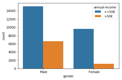
From the figure, we can infer that there are more number of males than females in the dataset. Next, we will use the bar graph to visualize the distribution of annual income based on both gender and hours per week (i.e. the number of hours they work per week).

# For this plot, we will be using the seaborn library as it provides more flexibility with dataframes.   
sns.barplot(data.gender, data['hours-per-week'], hue=data['annual-income'])  
plt.show()

So from the figure above, we can infer that males and females with annual income less than 50K tend to work more per week.

Countplot

This is a seaborn-specific function which is used to plot the count or frequency distribution of each unique observation in the categorical variable. It is similar to a histogram over a categorical rather than quantitative variable.

So, let’s plot the number of males and females in the dataset using the countplot function.

# Using Countplot to count number of males and females in the dataset.  
sns.countplot(data.gender)  
plt.show()  
count plot, seabormn data visualization, python, big data, machine leanring
Fig 3. Distribution of gender using countplot.

Earlier, we plotted the same thing using a bar graph, and it required some external calculations on our part to do so. But we can do the same thing using the countplot function in just a single line of code. Next, we will see how we can use countplot for deeper insights.

# ‘hue’ is used to visualize the effect of an additional variable to the current distribution.  
sns.countplot(data.gender, hue=data['annual-income'])  
plt.show()  
countplot, using hue, data visualization using seaborn
Fig 4. Distribution of gender based on annual income using countplot.

From the figure above, we can count that number of males and females whose annual income is <=50 and > 50K. We can see that the approximate number of

  • Males with annual income <=50K : 15,000
  • Males with annual income > 50K: 7000
  • Females with annual income <=50K: 9000
  • Females with annual income > 50K: 1000

So, we can infer that out of 32,500 (approx) people, only 8000 people have income greater than 50K, out of which only 1000 of them are females.

Machine learning challenge, ML challenge

Box plot

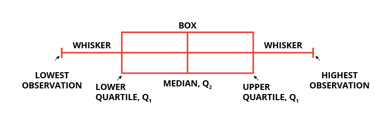
Box plots are widely used in data visualization. Box plots, also known as box and whisker plots are used to visualize variations and compare different categories in a given set of data. It doesn’t display the distribution in detail but is useful in detecting whether a distribution is skewed and detect outliers in the data. In a box and whisker plot:

  • the box spans the interquartile range
  • a vertical line inside the box represents the median
  • two lines outside the box, the whiskers, extending to the highest and the lowest observations represent the possible outliers in the data
whisker plot, box plot, seaborn, python, pyplot
Fig 5. Box and whisker plot.

Let’s use a box and whisker plot to find a correlation between ‘hours-per-week’ and ‘relationship’ based on their annual income.

# Creating a box plot  
fig, ax = plt.subplots(figsize=(15, 8))  
sns.boxplot(x='relationship', y='hours-per-week', hue='annual-income', data=data, ax=ax)  
ax.set_title('Annual Income of people based on relationship and hours-per-week')  
plt.show()  
box plot, whisker plot, visualization using box plot, box plot using seaborn, box plot in python
Fig 6. Using box plot to visualize how people in different relationships earn based on the number of hours they work per week.

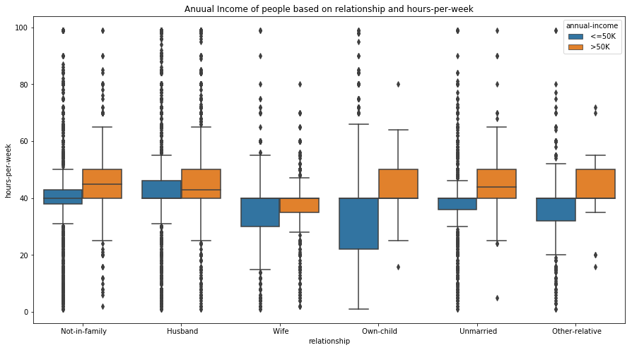
We can interpret some interesting results from the box plot. People with the same relationship status and an annual income more than 50K often work for more hours per week. Similarly, we can also infer that people who have a child and earn less than 50K tend to have more flexible working hours.
Apart from this, we can also detect outliers in the data. For example, people with relationship status ‘Not in family’ (see Fig 6.) and an income less than 50K have a large number of outliers at both the high and low ends. This also seems to be logically correct as a person who earns less than 50K annually may work more or less depending on the type of job and employment status.

Strip plot

Strip plot is a data analysis technique used to plot the sorted values of a variable along one axis. It is used to represent the distribution of a continuous variable with respect to the different levels of a categorical variable. For example, a strip plot can be used to show the distribution of the variable ‘gender’, i.e., males and females, with respect to the number of hours they work each week. A strip plot is also a good complement to a box plot or a violin plot in cases where you want to showcase all the observations along with some representation of the underlying distribution.

# Using Strip plot to visualize the data.  
fig, ax= plt.subplots(figsize=(10, 8))  
sns.stripplot(data['annual-income'], data['hours-per-week'], jitter=True, ax=ax)  
ax.set_title('Strip plot')  
plt.show()  
strip plot, strip plot using seaborn, strip plot in python, seaborn, python, machine learning, big data
Fig 7. Strip plot showing the distribution of the earnings based on the number of hours they work per week.

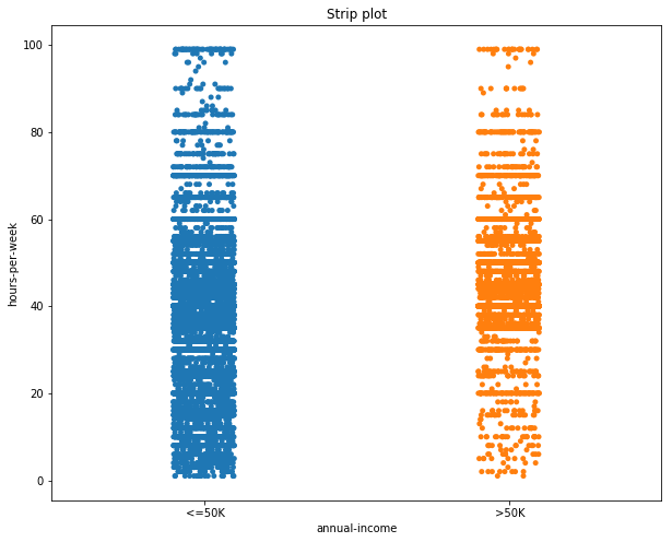
In the figure, by looking at the distribution of the data points, we can deduce that most of the people with an annual income greater than 50K work between 40 and 60 hours per week. While those with income less than 50K work can work between 0 and 60 hours per week.

Violin plot

Sometimes the mean and median may not be enough to understand the distribution of the variable in the dataset. The data may be clustered around the maximum or minimum with nothing in the middle. Box plots are a great way to summarize the statistical information related to the distribution of the data (through the interquartile range, mean, median), but they cannot be used to visualize the variations in the distributions.

A violin plot is a combination of a box plot and kernel density function (KDE, described in Part I of this blog series) which can be used to visualize the probability distribution of the data. Violin plots can be interpreted as follows:

  • The outer layer shows the probability distribution of the data points and indicates 95% confidence interval. The thicker the layer, the higher the probability of the data points, and vice-versa.
  • The second layer shows a box plot indicating the interquartile range.
  • The third layer, or the dot, indicates the median of the data.

    violin plot, interpreting a violin plot, how to read violin plot, violin plot in data visualization
    Fig 8. Representation of a violin plot.

Let’s now build a violin plot. To start with, we will analyze the distribution of annual income of the people w.r.t. the number of hours they work per week.

fig, ax = plt.subplots(figsize=(10, 8))  
sns.violinplot(x='annual-income', y='hours-per-week', data=data, ax=ax)  
ax.set_title('Violin plot')  
plt.show()  
violin plot, visualization using violin plot, violin plot using seaborn, how to plot using violin plot
Fig 9. Violin plot showing the distribution of the annual income based on the number of hours they work per week.

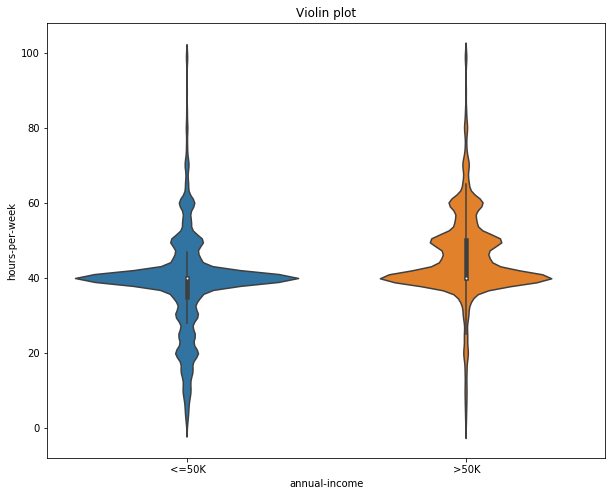
In Fig 9, the median number working hours per week is same (40 approximately) for both people earning less than 50K and greater than 50K. Although people earning less than 50K can have a varied range of the hours they spend working per week, most of the people who earn more than 50K work in the range of 40 – 80 hours per week.

Next, we can visualize the same distribution, but this grouping them according to their gender.

# Violin plot  
fig, ax = plt.subplots(figsize=(10, 8))  
sns.violinplot(x='annual-income', y='hours-per-week', hue='gender', data=data, ax=ax)  
ax.set_title('Violin plot grouped according to gender')  
plt.show()  
data visualization using violin plot, violin plot in seaborn, seaborn plots, plots in big data, plots in machine learning
Fig 10. Distribution of annual income based on the number of hours worked per week and gender.

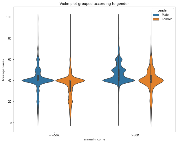
Adding the variable ‘gender’, gives us insights into how much each gender spends working per week based upon their annual income. From the figure, we can infer that males with annual income less than 50K tends to spend more hours working per week than females. But for people earning greater than 50K, both males and females spend an equal amount of hours per week working.

Violin plots, although more informative, are less frequently used in data visualization. It may be because they are hard to grasp and understand at first glance. But their ability to represent the variations in the data are making them popular among machine learning and data enthusiasts.

PairGrid

PairGrid is used to plot the pairwise relationship of all the variables in a dataset. This may seem to be similar to the pairplot we discussed in part I of this series. The difference is that instead of plotting all the plots automatically, as in the case of pairplot, Pair Grid creates a class instance, allowing us to map specific functions to the different sections of the grid.

Let’s start by defining the class.

# Creating an instance of the pair grid plot.  
g = sns.PairGrid(data=data, hue='annual-income')  

The variable ‘g’ here is a class instance. If we were to display ‘g’, then we will get a grid of empty plots. There are four grid sections to fill in a Pair Grid: upper triangle, lower triangle, the diagonal, and off-diagonal. To fill all the sections with the same plot, we can simply call ‘g.map’ with the type of plot and plot parameters.

# Creating a scatter plots for all pairs of variables.  
g = sns.PairGrid(data=data, hue='capital-gain')  
g.map(plt.scatter)  
data visualization using pair plot, visualizing multiple variabels, pair plot in seaborn, how to use pair plot
Fig 11. Scatter plot between each variable pair in the dataset.

The ‘g.map_lower’ method only fills the lower triangle of the grid while the ‘g.map_upper’ method only fills the upper triangle of the grid. Similarly, ‘g.map_diag’ and ‘g.map_offdiag’ fills the diagonal and off-diagonal of the grid, respectively.

#Here we plot scatter plot, histogram and violin plot using Pair grid.  
g = sns.PairGrid(data=data, vars = ['age', 'education-num', 'hours-per-week'])  
# with the help of the vars parameter we can select the variables between which we want the plot to be constructed.  

g.map_lower(plt.scatter, color='red')  
g.map_diag(plt.hist, bins=15)  
g.map_upper(sns.violinplot)  
data visualization using pair grid, how to use pair grid, pair grid, pair grid in seaborn, pair grid for big data
Fig 12. Pair Grid showing different plot between the different pair of variables.

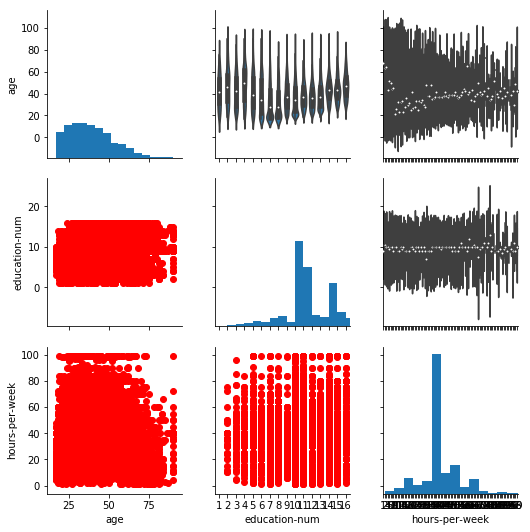
Thus with the help of Pair Grid, we can visualize the relationship between the three variables (‘hours-per-week’, ‘education-num’ and ‘age’) using three different plots all in the same figure. Pair grid comes in handy when visualizing multiple plots in the same figure.

Conclusion

Let’s summarize what we learned. So, we started with visualizing the distribution of categorical variables in isolation. Then, we moved on to visualize the relationship between a categorical and a continuous variable. Finally, we explored visualizing relationships when more than two variables are involved. Next week, we will explore how we can visualize unstructured data. Finally, I encourage you to download the given census data (used in this blog) or any other dataset of your choice and play with all the variations of the plots learned in this blog. Till then, Adiós!

Subscribe to The HackerEarth Blog

Get expert tips, hacks, and how-tos from the world of tech recruiting to stay on top of your hiring!

Author
Shubham Gupta
Calendar Icon
May 16, 2018
Timer Icon
3 min read
Share

Hire top tech talent with our recruitment platform

Access Free Demo
Related reads

Discover more articles

Gain insights to optimize your developer recruitment process.

The Mobile Dev Hiring Landscape Just Changed

Revolutionizing Mobile Talent Hiring: The HackerEarth Advantage

The demand for mobile applications is exploding, but finding and verifying developers with proven, real-world skills is more difficult than ever. Traditional assessment methods often fall short, failing to replicate the complexities of modern mobile development.

Introducing a New Era in Mobile Assessment

At HackerEarth, we're closing this critical gap with two groundbreaking features, seamlessly integrated into our Full Stack IDE:

Article content

Now, assess mobile developers in their true native environment. Our enhanced Full Stack questions now offer full support for both Java and Kotlin, the core languages powering the Android ecosystem. This allows you to evaluate candidates on authentic, real-world app development skills, moving beyond theoretical knowledge to practical application.

Article content

Say goodbye to setup drama and tool-switching. Candidates can now build, test, and debug Android and React Native applications directly within the browser-based IDE. This seamless, in-browser experience provides a true-to-life evaluation, saving valuable time for both candidates and your hiring team.

Assess the Skills That Truly Matter

With native Android support, your assessments can now delve into a candidate's ability to write clean, efficient, and functional code in the languages professional developers use daily. Kotlin's rapid adoption makes proficiency in it a key indicator of a forward-thinking candidate ready for modern mobile development.

Breakup of Mobile development skills ~95% of mobile app dev happens through Java and Kotlin
This chart illustrates the importance of assessing proficiency in both modern (Kotlin) and established (Java) codebases.

Streamlining Your Assessment Workflow

The integrated mobile emulator fundamentally transforms the assessment process. By eliminating the friction of fragmented toolchains and complex local setups, we enable a faster, more effective evaluation and a superior candidate experience.

Old Fragmented Way vs. The New, Integrated Way
Visualize the stark difference: Our streamlined workflow removes technical hurdles, allowing candidates to focus purely on demonstrating their coding and problem-solving abilities.

Quantifiable Impact on Hiring Success

A seamless and authentic assessment environment isn't just a convenience, it's a powerful catalyst for efficiency and better hiring outcomes. By removing technical barriers, candidates can focus entirely on demonstrating their skills, leading to faster submissions and higher-quality signals for your recruiters and hiring managers.

A Better Experience for Everyone

Our new features are meticulously designed to benefit the entire hiring ecosystem:

For Recruiters & Hiring Managers:

  • Accurately assess real-world development skills.
  • Gain deeper insights into candidate proficiency.
  • Hire with greater confidence and speed.
  • Reduce candidate drop-off from technical friction.

For Candidates:

  • Enjoy a seamless, efficient assessment experience.
  • No need to switch between different tools or manage complex setups.
  • Focus purely on showcasing skills, not environment configurations.
  • Work in a powerful, professional-grade IDE.

Unlock a New Era of Mobile Talent Assessment

Stop guessing and start hiring the best mobile developers with confidence. Explore how HackerEarth can transform your tech recruiting.

Vibe Coding: Shaping the Future of Software

A New Era of Code

Vibe coding is a new method of using natural language prompts and AI tools to generate code. I have seen firsthand that this change makes software more accessible to everyone. In the past, being able to produce functional code was a strong advantage for developers. Today, when code is produced quickly through AI, the true value lies in designing, refining, and optimizing systems. Our role now goes beyond writing code; we must also ensure that our systems remain efficient and reliable.

From Machine Language to Natural Language

I recall the early days when every line of code was written manually. We progressed from machine language to high-level programming, and now we are beginning to interact with our tools using natural language. This development does not only increase speed but also changes how we approach problem solving. Product managers can now create working demos in hours instead of weeks, and founders have a clearer way of pitching their ideas with functional prototypes. It is important for us to rethink our role as developers and focus on architecture and system design rather than simply on typing c

The Promise and the Pitfalls

I have experienced both sides of vibe coding. In cases where the goal was to build a quick prototype or a simple internal tool, AI-generated code provided impressive results. Teams have been able to test new ideas and validate concepts much faster. However, when it comes to more complex systems that require careful planning and attention to detail, the output from AI can be problematic. I have seen situations where AI produces large volumes of code that become difficult to manage without significant human intervention.

AI-powered coding tools like GitHub Copilot and AWS’s Q Developer have demonstrated significant productivity gains. For instance, at the National Australia Bank, it’s reported that half of the production code is generated by Q Developer, allowing developers to focus on higher-level problem-solving . Similarly, platforms like Lovable enable non-coders to build viable tech businesses using natural language prompts, contributing to a shift where AI-generated code reduces the need for large engineering teams. However, there are challenges. AI-generated code can sometimes be verbose or lack the architectural discipline required for complex systems. While AI can rapidly produce prototypes or simple utilities, building large-scale systems still necessitates experienced engineers to refine and optimize the code.​

The Economic Impact

The democratization of code generation is altering the economic landscape of software development. As AI tools become more prevalent, the value of average coding skills may diminish, potentially affecting salaries for entry-level positions. Conversely, developers who excel in system design, architecture, and optimization are likely to see increased demand and compensation.​
Seizing the Opportunity

Vibe coding is most beneficial in areas such as rapid prototyping and building simple applications or internal tools. It frees up valuable time that we can then invest in higher-level tasks such as system architecture, security, and user experience. When used in the right context, AI becomes a helpful partner that accelerates the development process without replacing the need for skilled engineers.

This is revolutionizing our craft, much like the shift from machine language to assembly to high-level languages did in the past. AI can churn out code at lightning speed, but remember, “Any fool can write code that a computer can understand. Good programmers write code that humans can understand.” Use AI for rapid prototyping, but it’s your expertise that transforms raw output into robust, scalable software. By honing our skills in design and architecture, we ensure our work remains impactful and enduring. Let’s continue to learn, adapt, and build software that stands the test of time.​

Ready to streamline your recruitment process? Get a free demo to explore cutting-edge solutions and resources for your hiring needs.

Guide to Conducting Successful System Design Interviews in 2025

What is Systems Design?

Systems Design is an all encompassing term which encapsulates both frontend and backend components harmonized to define the overall architecture of a product.

Designing robust and scalable systems requires a deep understanding of application, architecture and their underlying components like networks, data, interfaces and modules.

Systems Design, in its essence, is a blueprint of how software and applications should work to meet specific goals. The multi-dimensional nature of this discipline makes it open-ended – as there is no single one-size-fits-all solution to a system design problem.

What is a System Design Interview?

Conducting a System Design interview requires recruiters to take an unconventional approach and look beyond right or wrong answers. Recruiters should aim for evaluating a candidate’s ‘systemic thinking’ skills across three key aspects:

How they navigate technical complexity and navigate uncertainty
How they meet expectations of scale, security and speed
How they focus on the bigger picture without losing sight of details

This assessment of the end-to-end thought process and a holistic approach to problem-solving is what the interview should focus on.

What are some common topics for a System Design Interview

System design interview questions are free-form and exploratory in nature where there is no right or best answer to a specific problem statement. Here are some common questions:

How would you approach the design of a social media app or video app?

What are some ways to design a search engine or a ticketing system?

How would you design an API for a payment gateway?

What are some trade-offs and constraints you will consider while designing systems?

What is your rationale for taking a particular approach to problem solving?

Usually, interviewers base the questions depending on the organization, its goals, key competitors and a candidate’s experience level.

For senior roles, the questions tend to focus on assessing the computational thinking, decision making and reasoning ability of a candidate. For entry level job interviews, the questions are designed to test the hard skills required for building a system architecture.

The Difference between a System Design Interview and a Coding Interview

If a coding interview is like a map that takes you from point A to Z – a systems design interview is like a compass which gives you a sense of the right direction.

Here are three key difference between the two:

Coding challenges follow a linear interviewing experience i.e. candidates are given a problem and interaction with recruiters is limited. System design interviews are more lateral and conversational, requiring active participation from interviewers.

Coding interviews or challenges focus on evaluating the technical acumen of a candidate whereas systems design interviews are oriented to assess problem solving and interpersonal skills.

Coding interviews are based on a right/wrong approach with ideal answers to problem statements while a systems design interview focuses on assessing the thought process and the ability to reason from first principles.

How to Conduct an Effective System Design Interview

One common mistake recruiters make is that they approach a system design interview with the expectations and preparation of a typical coding interview.
Here is a four step framework technical recruiters can follow to ensure a seamless and productive interview experience:

Step 1: Understand the subject at hand

  • Develop an understanding of basics of system design and architecture
  • Familiarize yourself with commonly asked systems design interview questions
  • Read about system design case studies for popular applications
  • Structure the questions and problems by increasing magnitude of difficulty

Step 2: Prepare for the interview

  • Plan the extent of the topics and scope of discussion in advance
  • Clearly define the evaluation criteria and communicate expectations
  • Quantify constraints, inputs, boundaries and assumptions
  • Establish the broader context and a detailed scope of the exercise

Step 3: Stay actively involved

  • Ask follow-up questions to challenge a solution
  • Probe candidates to gauge real-time logical reasoning skills
  • Make it a conversation and take notes of important pointers and outcomes
  • Guide candidates with hints and suggestions to steer them in the right direction

Step 4: Be a collaborator

  • Encourage candidates to explore and consider alternative solutions
  • Work with the candidate to drill the problem into smaller tasks
  • Provide context and supporting details to help candidates stay on track
  • Ask follow-up questions to learn about the candidate’s experience

Technical recruiters and hiring managers should aim for providing an environment of positive reinforcement, actionable feedback and encouragement to candidates.

Evaluation Rubric for Candidates

Facilitate Successful System Design Interview Experiences with FaceCode

FaceCode, HackerEarth’s intuitive and secure platform, empowers recruiters to conduct system design interviews in a live coding environment with HD video chat.

FaceCode comes with an interactive diagram board which makes it easier for interviewers to assess the design thinking skills and conduct communication assessments using a built-in library of diagram based questions.

With FaceCode, you can combine your feedback points with AI-powered insights to generate accurate, data-driven assessment reports in a breeze. Plus, you can access interview recordings and transcripts anytime to recall and trace back the interview experience.

Learn how FaceCode can help you conduct system design interviews and boost your hiring efficiency.

Top Products

Explore HackerEarth’s top products for Hiring & Innovation

Discover powerful tools designed to streamline hiring, assess talent efficiently, and run seamless hackathons. Explore HackerEarth’s top products that help businesses innovate and grow.
Frame
Hackathons
Engage global developers through innovation
Arrow
Frame 2
Assessments
AI-driven advanced coding assessments
Arrow
Frame 3
FaceCode
Real-time code editor for effective coding interviews
Arrow
Frame 4
L & D
Tailored learning paths for continuous assessments
Arrow
Get A Free Demo